8.2 Evidence of past glaciation
Outline:
The last glacial maximum
The Cordilleran ice sheet
Evidence of glacial flow direction
Additional Assigned Reading
Physical Geology – 2nd Edition, By Steven Earle Chapter 16 Glaciation
Listen to this episode of the podcast Bay Curious about “The Bay Area During the Ice Age”
The Last Glacial Maximum
Around 20,000 years ago was the last glacial maximum, the most recent of glacial intervals associated with climate going between a glacial and interglacial climate states over the past 2.5 million years. We will look at data associated with more of these cycles when we talk about time-series analysis. For the moment, let’s focus on the warming from the last glacial maximum which is visualized (based on estimates published in a couple different scientific papers) in the following xkcd comic:

At the last glacial maximum, the extent of ice sheets on North America were the following such that nearly all of Canada was covered in an ice sheet (like Greenland is today) with this ice sheet extending down into the lower 48 states of the present-day United States:
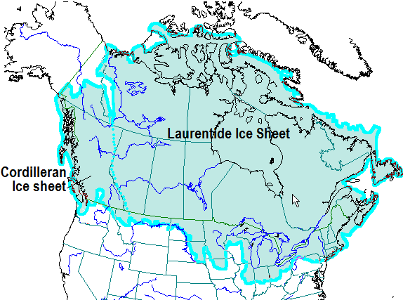
Source https://opentextbc.ca/geology/chapter/16-1-glacial-periods-in-earths-history/
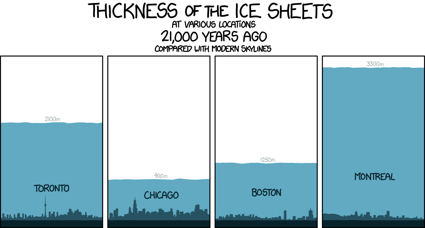
This xkcd comic is a helpful visualization of the thickness of the Laurentide ice sheet at the location of a few modern day cities:
The Cordilleran ice sheet
Let’s focus on the Cordilleran ice sheet which is visualized here:
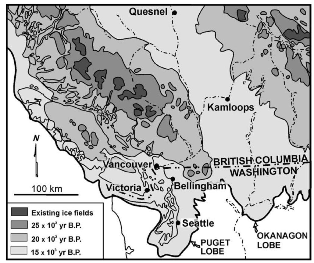
Source Booth et al. 2003 where it is modified from Clague (1981)
Booth et al. (2003) in their review paper on the Cordilleran ice sheet provide this summary of the history of the most recent growth of the ice sheet.
The Cordilleran ice sheet most recently advanced out of the mountains of British Columbia about 25,000 14C yr B.P. It flowed west onto the continental shelf, east into the intermontaine valleys of British Columbia where it probably merged with the western edge of the Laurentide ice sheet, and south into the lowlands of Washington State (Fig. 8, Table 1). In southern British Columbia and western Washington the Puget lobe filled the Fraser Lowland and the Puget Lowland between the Olympic Mountains and Cascade Range. The Juan de Fuca lobe extended east along the Strait of Juan de Fuca to termine some 100km west of Washington’s present coast. Several ice lobes east of the Cascade Range expanded south down the Okanogan Valley and down other valleys farther east. The Fraser-age ice-sheet maximum on both sides of the Cascade Range was broadly synchronous (Waitt & Thorson, 1983). It approximately coincided with the maximum advance of some parts of the Laurentide ice sheet in central North America at about 14,000 14C yr B.P. but lagged several thousand years behind the culminating advance of the most of the Laurentide ice sheet (Lowell et al., 1999; Mickelson et al., 1983; Prest, 1969). *The cordilleran ice sheet, Booth et al. 2003
There are a lot of different statements made in the above summary paragraph that come from a lot of different data types. For today, let’s focus on the statements regarding the flow direction.
This photograph of the Aletsch Glacier in Switzerland provides a striking visualization of ice flow in a modern glacier as detritus associated with rock falls onto the glacier have been stretched out in the direction of ice flow:
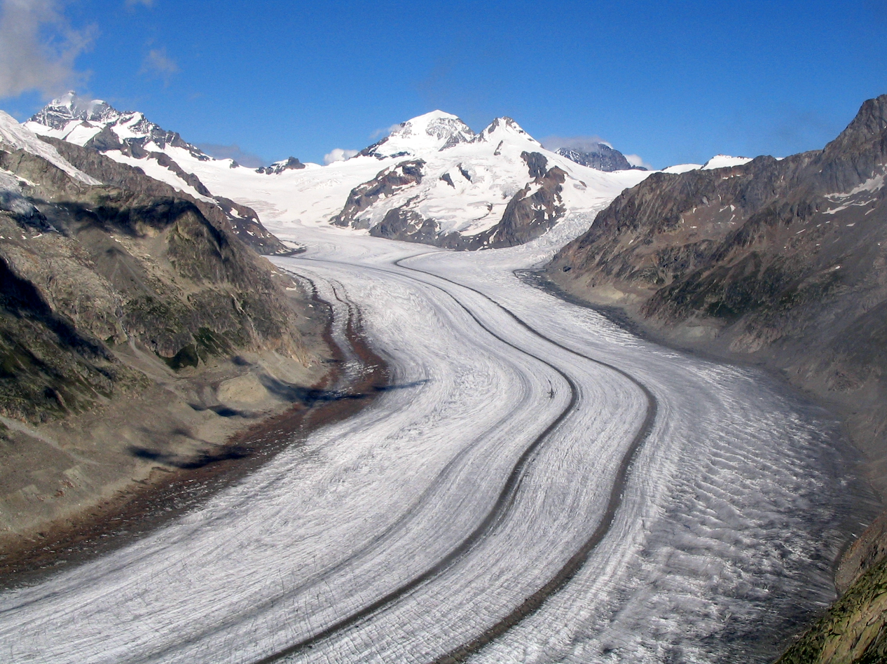
The Aletsch Glacier, the largest glacier of the Alps, in Switzerland. Source: By Dirk Beyer - Own work, CC BY-SA 3.0, https://commons.wikimedia.org/w/index.php?curid=352940
How do Earth scientists determine the extent and direction of ice sheet flow?
As covered in Chapter 16 of Physical Geology, the presence of ice lead to a number of different types of features.
Striation & Striation or groove
As glaciers flow, they can entrain rocks. If these rocks come in contact with the base of the glacier, they can scratch the underlying rock resulting in striations or scouring out larger-scale grooves:
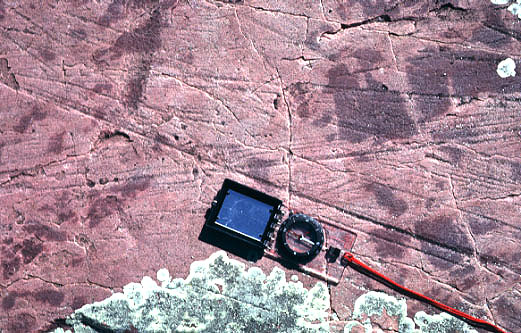
Photograph of glacial striations and grooves on Sioux Quartzite bedrock at Jeffers, Minnesota. At least two directions of ice movement are indicated by crossing (x) pattern of striae. Source: http://academic.emporia.edu/aberjame/ice/lec01/lec1.htm.
Crag-and-tail
Definition: a tadpole-shaped landform developed by glacial erosion of rocks on unequal resistance. The crags are cliffs developed in near-cylindrical masses of strong rock. The tail is formed in softer rocks sheltered from erosion in its lee. Source: http://www.landforms.eu/Lothian/crag%20and%20tail.htm
This image from Victoria Island in British Columbia shows both striations and miniture crag-and-tail features:
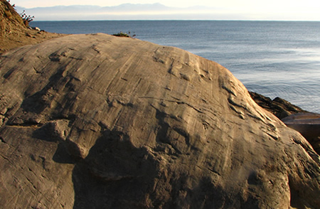
Source: https://www.geocaching.com/geocache/GC1HW85_victoria-earthcache-series-3-all-scratched-up
Crag-and-tail features can also be much larger such as Abbey Craig, a hilltop overlooking Stirling in Scotland on which a monument to Sir William Wallace was built.
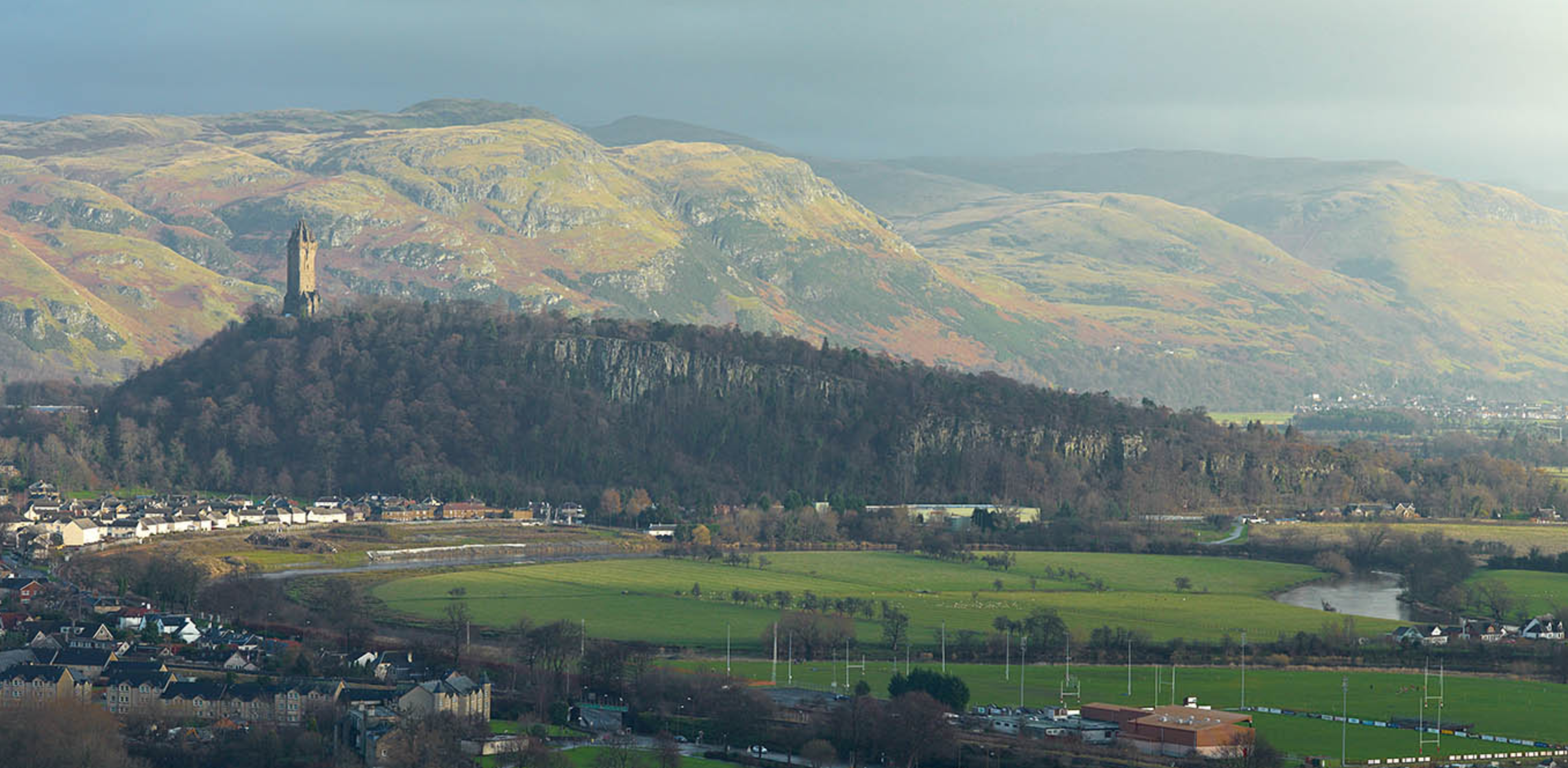
Source: http://lenstalk.com/index.php/albumscotland/album01/album22/album24/L1000139_Abbey_Craig_and_the_Ochils_from_Stirling_Castle
Drumlin, Drumlinoid, Fluted bedrock & fluting
Drumlin definition: An elongate hill, streamlined in the direction of ice flow and composed largely of glacial deposits.
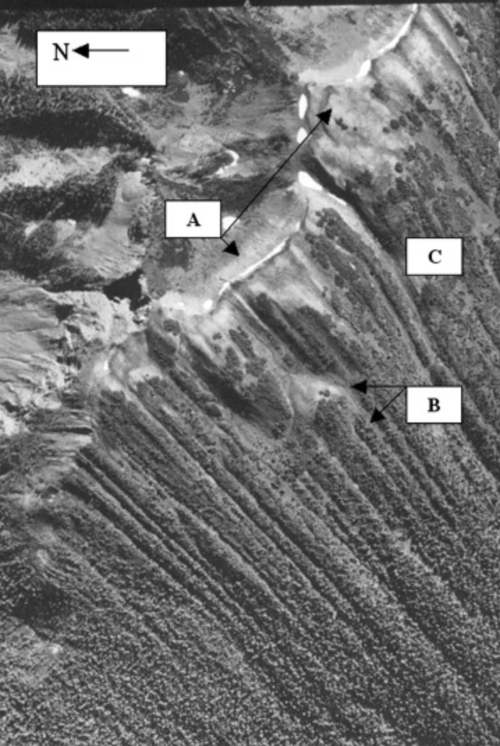
Airphoto of Drumlins on Hazelton Peak [British Columbia]. Flow is toward the bottom right of the photo. Some of the stoss (upflow) ends of the drumlins are truncated by cliff faces (A). Stoss-end crescentic furrows are visible that merge with lateral furrows separating the drumlins, thus producing U-shaped furrows (B). Source: Streamlined erosional residuals and drumlins in central British Columbia McClenagan (2013) https://doi.org/10.1016/j.geomorph.2013.01.015
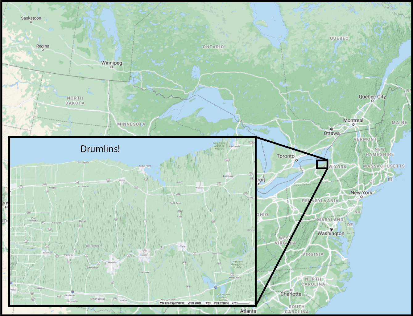
I grew up on a drumlin!!! Here are some a good examples from Western New York.
Directional Data
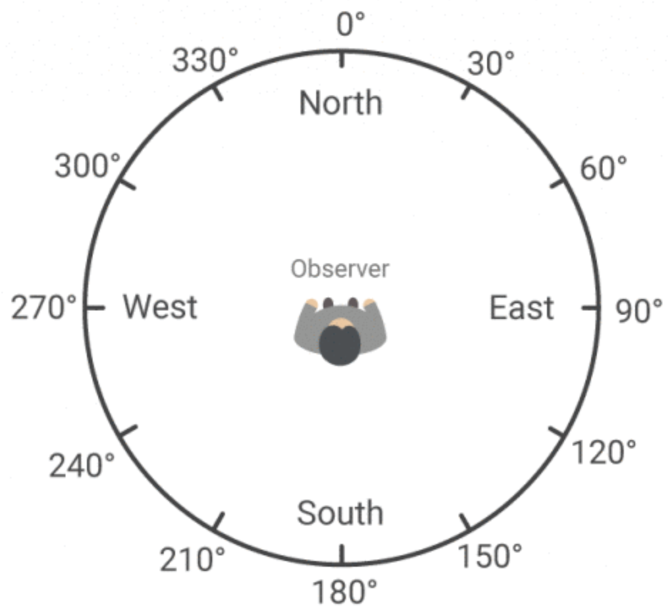
Azimuth
Earth science is filled with directional data. The most typical way that directional data are reported is as azimuth:
Getting the x length and y length of the unit vector associated with the azimuth
If \(\theta=0\)° \(sin(\theta)=1\) and \(cos(\theta)=0\)
If \(\theta=90\)° \(sin(\theta)=0\) and \(cos(\theta)=1\)
If \(\theta=225\)° \(sin(\theta)= -0.7071\) and \(cos(\theta)= -0.7071\)
Unfortunately, the trignometric convention is rotated 90° from the geographic convention, but the result is that:
x_length = sin(azimuth)
y_length = cos(azimuth)

Visualizing the directions
Quiver map
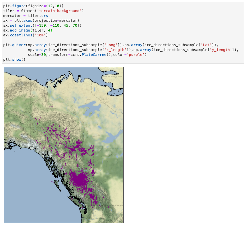
We can represent our directions as arrows (quivers) mapped at the geographic location where the data was collected using matplotlibs’ plt.quiver.
We will follow these steps:
For quiver maps, we will create a map projection instance (called
ax) with theax = plt.axes(projection=)function.As we have done with earlier maps we set the edges of our map with
ax.set_extent([])and add coastlines and a background image if wanted withax.add_image()andax.coastlines().We will use
plt.quiver()to add the data to the map. The data needs to be input as numpy arrays. First the positions of the arrows are given with the longitude and latitude arrays. Then the arrow properties are input - their x-component lengths and y-component lengths. Then as with other map plots we need to settransform=ccrs.PlateCarree(). The color and scale of the arrows can be set to make a nice looking map.
Rose diagrams
Text modified from Lisa Tauxe’s materials for her Python for Earth Science Students course: https://github.com/ltauxe/Python-for-Earth-Science-Students
As Earth scientists, we like to make plots that convey the most information with the least amount of effort for the viewer. 2D directional data are much better represented as ‘rose diagrams’, which are really just histograms plotted around a circle. They are also known as polar projections as they could be used to make a map of the Earth looking down at one of the poles.
We will follow these steps:
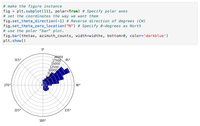
For rose diagrams, we will create a plot instance (called
fig) with theplt.subplot( )function. We make it a polar plot by setting thepolarkeyword toTrue.The polar type of subplot has funny coordinates set as default, funny to an Earth scientist at least. The orientations go around counterclockwise instead of clockwise (like map directions). To make it seem more normal for Earth science data, we have to switch around the directions to geographic coordinates. We do this with the fig.set_theta_direction(-1) function where the ‘-1’ tells matplotlib that we want the numbers to go around clockwise, instead of the default (which for some unknown reason goes counter clockwise).
We also have to put ‘0’ at the top of the diagram (because it is ‘North’ in Earth science). We do that with the
fig.set_theta_zero_location('N')call, which tellsmatplotlibto put 0 on top (instead of on the right side which is the default).We have to define some bins, sort of like histograms but around azimuthal circle, and count up how many directions are in each bin. We will use a bin size of 10$^{\circ}$. Fortunately,
plt.hist( )will count up the number of directional data in each bin for us! Usually we just useplt.hist()to make the plot, but we can also have it return the bins and the number in each bin.We will use the plot function plt.bar( ) which normally makes bar charts, but will make rose diagrams if the plot is polar.
Finally, we will plot the data on the figure instance.