11.1 Machine learning: Clustering and Classification
Outline:
Machine learning
Classification, regression, clustering
Training set and test set
Additional Assigned Reading
Data 8 textbook “Computational and Inferential Thinking: The Foundations of Data Science” By Ani Adhikari and John DeNero Chapter 17 Classificiation. This should overlap with your assigned reading for Data 8.
Machine learning
Text from: https://scikit-learn.org/stable/tutorial/basic/tutorial.html
In general, a learning problem considers a set of \(n\) samples of data and then tries to predict properties of unknown data. If each sample is more than a single number and, for instance, a multi-dimensional entry (aka multivariate data), it is said to have several attributes or features.
Learning problems fall into a few categories:
supervised learning, in which the data comes with additional attributes that we want to predict (Click here to go to the scikit-learn supervised learning page).This problem can be either: - classification: samples belong to two or more classes and we want to learn from already labeled data how to predict the class of unlabeled data. An example of a classification problem would be handwritten digit recognition, in which the aim is to assign each input vector to one of a finite number of discrete categories. Another way to think of classification is as a discrete (as opposed to continuous) form of supervised learning where one has a limited number of categories and for each of the n samples provided, one is to try to label them with the correct category or class. - regression: if the desired output consists of one or more continuous variables, then the task is called regression. An example of a regression problem would be the prediction of the length of a salmon as a function of its age and weight.
unsupervised learning, in which the training data consists of a set of input vectors \(x\) without any corresponding target values. The goal in such problems may be to discover groups of similar examples within the data, where it is called clustering, or to determine the distribution of data within the input space, known as density estimation, or to project the data from a high-dimensional space down to two or three dimensions for the purpose of visualization (Click here to go to the Scikit-Learn unsupervised learning page).
Training set and testing set
Machine learning is about learning some properties of a data set and then testing those properties against another data set. A common practice in machine learning is to evaluate an algorithm by splitting a data set into two. We call one of those sets the training set, on which we learn some properties; we call the other set the testing set, on which we test the learned properties.
Classification algorithms
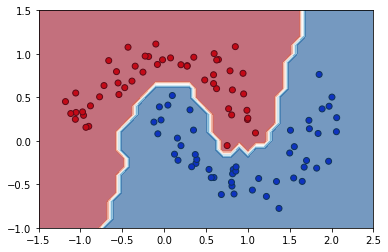
Here is an example of a nearest neighbor classifier, which classifies a point based on its nearest \(k=3\) observation point, similar to the one done in the Data 8 text using the scikit-learn funtions.
import numpy as np
import matplotlib.pyplot as plt
from matplotlib.colors import ListedColormap
from sklearn.datasets import make_moons
from sklearn.neighbors import KNeighborsClassifier

X,y = make_moons(100,noise=0.15)

cm = plt.cm.RdBu
cm_bright = ListedColormap(['#FF0000', '#0000FF'])

# setup the classifier algorithm and fit to observations
neigh = KNeighborsClassifier(n_neighbors=3, weights='distance')
neigh.fit(X,y)

# predict classification of points on a grid
xx, yy = np.meshgrid(np.arange(-1.5, 2.6, 0.1),np.arange(-1, 1.6, 0.1))
Z = neigh.predict(np.c_[xx.ravel(), yy.ravel()])

# plot observations
plt.scatter(X[:, 0], X[:, 1], c=y, cmap=cm_bright,edgecolors='k')
# plot the predictions
Z = Z.reshape(xx.shape)
plt.contourf(xx, yy, Z, cmap=cm, alpha=.6)
plt.show()
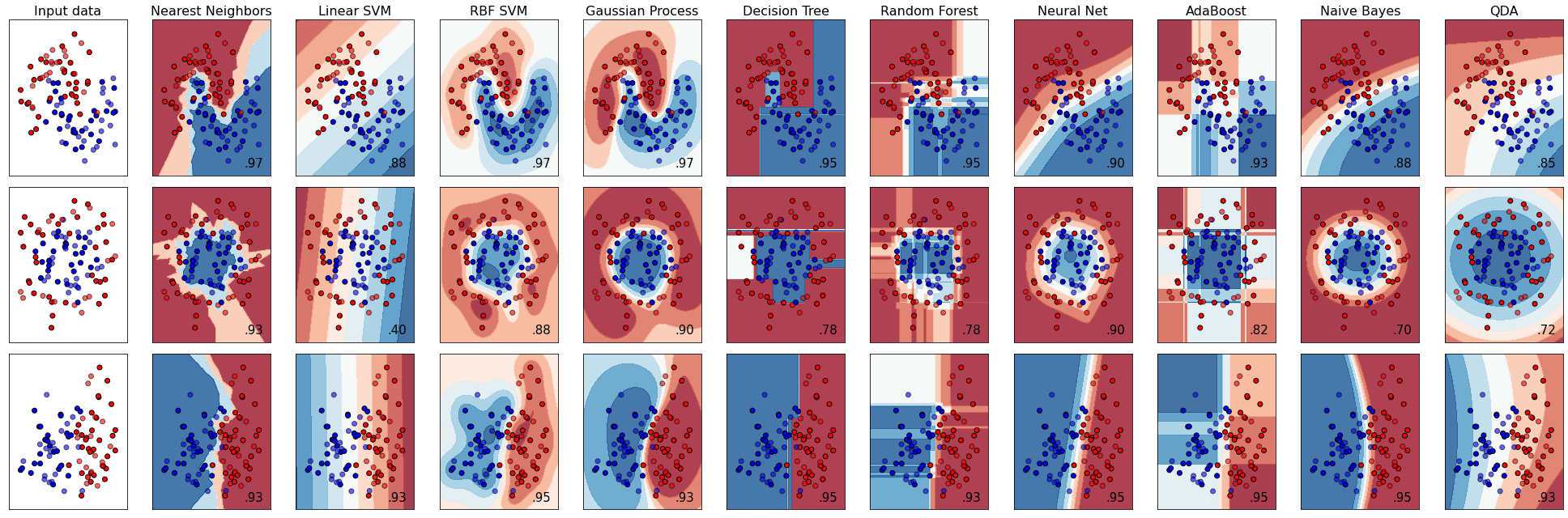
If you go to the scikit-learn homepage you will find many available classifiers: https://scikit-learn.org/stable/index.html. They are nicely illustrated in this code from the scikit-learn documentation. Different algorithms will be suitable for different situations.
# Code source: Gaël Varoquaux
#              Andreas Müller
# Modified for documentation by Jaques Grobler
# License: BSD 3 clause

import numpy as np
import matplotlib.pyplot as plt
from matplotlib.colors import ListedColormap
from sklearn.model_selection import train_test_split
from sklearn.preprocessing import StandardScaler
from sklearn.datasets import make_moons, make_circles, make_classification
from sklearn.neural_network import MLPClassifier
from sklearn.neighbors import KNeighborsClassifier
from sklearn.svm import SVC
from sklearn.gaussian_process import GaussianProcessClassifier
from sklearn.gaussian_process.kernels import RBF
from sklearn.tree import DecisionTreeClassifier
from sklearn.ensemble import RandomForestClassifier, AdaBoostClassifier
from sklearn.naive_bayes import GaussianNB
from sklearn.discriminant_analysis import QuadraticDiscriminantAnalysis

h = .02  # step size in the mesh

names = ["Nearest Neighbors", "Linear SVM", "RBF SVM", "Gaussian Process",
         "Decision Tree", "Random Forest", "Neural Net", "AdaBoost",
         "Naive Bayes", "QDA"]

classifiers = [
    KNeighborsClassifier(3),
    SVC(kernel="linear", C=0.025),
    SVC(gamma=2, C=1),
    GaussianProcessClassifier(1.0 * RBF(1.0)),
    DecisionTreeClassifier(max_depth=5),
    RandomForestClassifier(max_depth=5, n_estimators=10, max_features=1),
    MLPClassifier(alpha=1, max_iter=1000),
    AdaBoostClassifier(),
    GaussianNB(),
    QuadraticDiscriminantAnalysis()]

X, y = make_classification(n_features=2, n_redundant=0, n_informative=2,
                           random_state=1, n_clusters_per_class=1)
rng = np.random.RandomState(2)
X += 2 * rng.uniform(size=X.shape)
linearly_separable = (X, y)

datasets = [make_moons(noise=0.3, random_state=0),
            make_circles(noise=0.2, factor=0.5, random_state=1),
            linearly_separable
            ]

figure = plt.figure(figsize=(27, 9))
i = 1
# iterate over datasets
for ds_cnt, ds in enumerate(datasets):
    # preprocess dataset, split into training and test part
    X, y = ds
    X = StandardScaler().fit_transform(X)
    X_train, X_test, y_train, y_test = \
        train_test_split(X, y, test_size=.4, random_state=42)

    x_min, x_max = X[:, 0].min() - .5, X[:, 0].max() + .5
    y_min, y_max = X[:, 1].min() - .5, X[:, 1].max() + .5
    xx, yy = np.meshgrid(np.arange(x_min, x_max, h),
                         np.arange(y_min, y_max, h))

    # just plot the dataset first
    cm = plt.cm.RdBu
    cm_bright = ListedColormap(['#FF0000', '#0000FF'])
    ax = plt.subplot(len(datasets), len(classifiers) + 1, i)
    if ds_cnt == 0:
        ax.set_title("Input data", fontsize = 16)
    # Plot the training points
    ax.scatter(X_train[:, 0], X_train[:, 1], c=y_train, cmap=cm_bright,
               edgecolors='k')
    # Plot the testing points
    ax.scatter(X_test[:, 0], X_test[:, 1], c=y_test, cmap=cm_bright, alpha=0.6,
               edgecolors='k')
    ax.set_xlim(xx.min(), xx.max())
    ax.set_ylim(yy.min(), yy.max())
    ax.set_xticks(())
    ax.set_yticks(())
    i += 1

    # iterate over classifiers
    for name, clf in zip(names, classifiers):
        ax = plt.subplot(len(datasets), len(classifiers) + 1, i)
        clf.fit(X_train, y_train)
        score = clf.score(X_test, y_test)

        # Plot the decision boundary. For that, we will assign a color to each
        # point in the mesh [x_min, x_max]x[y_min, y_max].
        if hasattr(clf, "decision_function"):
            Z = clf.decision_function(np.c_[xx.ravel(), yy.ravel()])
        else:
            Z = clf.predict_proba(np.c_[xx.ravel(), yy.ravel()])[:, 1]

        # Put the result into a color plot
        Z = Z.reshape(xx.shape)
        ax.contourf(xx, yy, Z, cmap=cm, alpha=.8)

        # Plot the training points
        ax.scatter(X_train[:, 0], X_train[:, 1], c=y_train, cmap=cm_bright,
                   edgecolors='k')
        # Plot the testing points
        ax.scatter(X_test[:, 0], X_test[:, 1], c=y_test, cmap=cm_bright,
                   edgecolors='k', alpha=0.6)

        ax.set_xlim(xx.min(), xx.max())
        ax.set_ylim(yy.min(), yy.max())
        ax.set_xticks(())
        ax.set_yticks(())
        if ds_cnt == 0:
            ax.set_title(name, fontsize=16)
        ax.text(xx.max() - .3, yy.min() + .3, ('%.2f' % score).lstrip('0'),
                size=15, horizontalalignment='right')
        i += 1

plt.tight_layout()
plt.show()